

1. Introduction
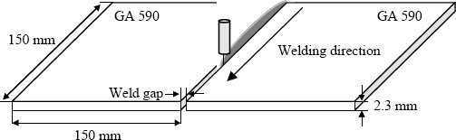
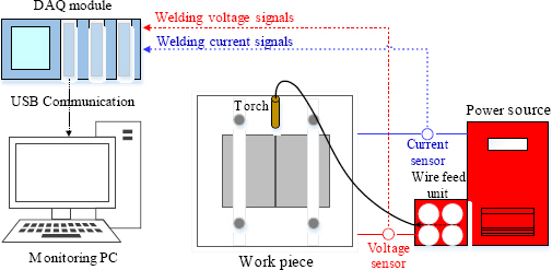
2. Experimental Procedures
Table┬Ā1
| GA 590 | Chemical compositions (wt%) | mechanical properties | |||||||
| C | Mn | Si | S | P | Fe | YS (MPa) | TS (MPa) | EI (%) | |
| 0.0825 | 1.440 | 0.132 | 0.002 | 0.011 | Bal | 583 | 628 | 25 | |
3. Results and Analysis
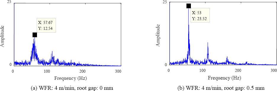
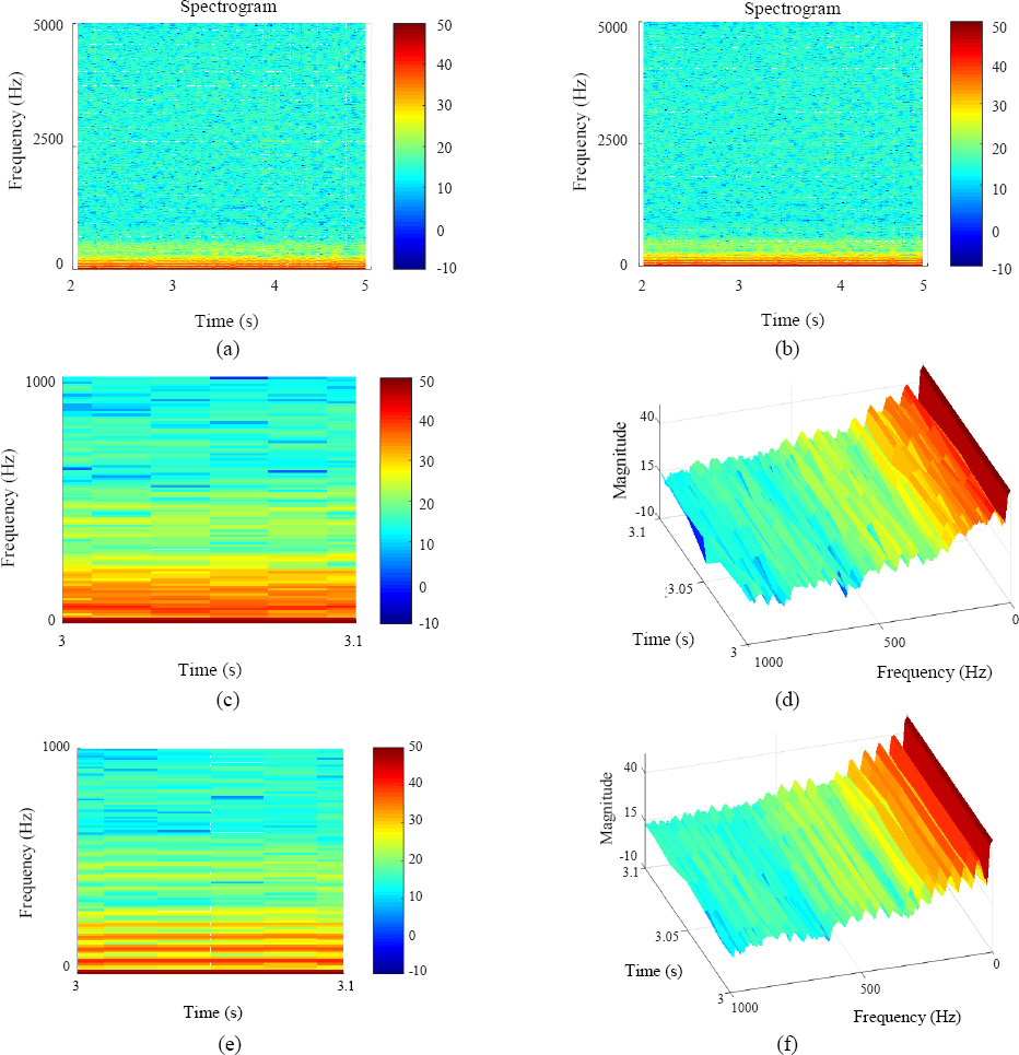
3.1 Welding Current Signal Analysis Using STFT
Fig.┬Ā3

Fig.┬Ā4
3.2 CNN Theory and Performance Evaluation
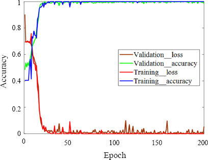
3.2.1 Training process

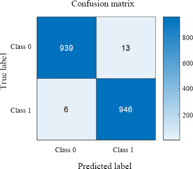
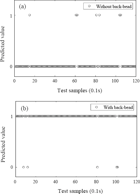
3.2.2 Testing process
Fig.┬Ā9
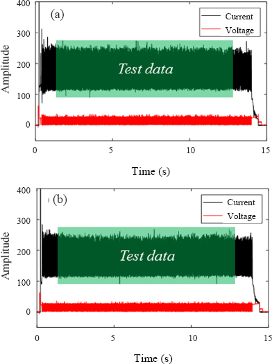
Fig.┬Ā10
Table┬Ā3
| Variable | Validation samples | Estimated | Error | Accuracy |
|---|---|---|---|---|
| Class 0 | 952 | 939 | 13 | 98.6 % |
| Class 1 | 952 | 946 | 6 | 99.3 % |
Table┬Ā4
| Variable | Test samples | Estimated | Error | Accuracy |
|---|---|---|---|---|
| Class 0 | 120 | 113 | 7 | 94.2 % |
| Class 1 | 120 | 115 | 5 | 95.8 % |
4. Conclusion
1) In this study, the spectrogram image obtained by the STFT frequency conversion was extracted by measuring the welding current generated in the GMAW process, and it was trained and validated by labeling with 0 and 1 classes indicating whether or not a bead was formed
2) The difference in the shape of the spectrogram image acquired in the time-frequency domain transform with and without back-bead formation was identified, and the input spectrogram image was visualized as a feature map formed in each layer of CNN to show the difference between the shape of the feature map with and without back-bead.
3) The prediction performance of the proposed CNN model was verified, and the detection performance was 95.8 % and 94.2 % for the regions with and without back-bead, respectively, as a result of applying it to a new welding data.
 PDF Links
 PubReader
 ePub Link
 Full text via DOI
 Download Citation
 Print
Print


