1. Introduction
Welding simulations are state of the art and carried out on a large scale for 1-D seams. These are used in the industrial environment for the estimation of process variables and their effects. The advantage of digital application is that time and costs can be saved by reducing the number of bench tests. Furthermore, it is possible to investigate phenomena, such as thermal behavior or the resulting deformation, that could only be observed at great expense or not at all
1-4).
The understanding of these thermal phenomena can be used to adapt weld parameters in advance to avoid defects, in particular for 2-D welds. However simulations of welding processes at 2-D seams are available to a rather small extent. Temperature fields during welding of pipes are determined
5,6). Also heat sources that are guided spirally around the pipe have been investigated
7).
Generally thermal numerical analysis are used to predict deformation and residual stresses
7-9). Also the evaluation of effects from laser beam power, welding speed and beam angle, such as the width and depth of molten pool at T-joints is predicted
10).
Besides the simulative mapping, the setup of a system for setting the welding parameters with an artificial neural network as a prediction tool is used. This tool performs a non-linear mapping between inputs and outputs of a 1-D welding process
11). Such an approach could also be used to adapt welding parameters for changing boundary conditions.
In this work temperature fields of 2-D Tjoints are to be generated in the radius. These temperature fields, which are generated by FEA, are used to estimate the necessary power adjustment for real welding trials. This should serve as a basis for a systematic approach to avoid failures, based on heat accumulation. In the future, it should be possible to obtain laser power automatically in offline programming, also for 3-D welding applications, or to use power adjustments as a baseline for other welding parameter investigations.
2. Used welding setup
The setup is comprised of an articulated robot and a Fronius laser hybrid welding head, with an integrated Trans Puls Synergic welding system. The laser source is an IPG YLR-5000 fiber laser, with a Trumpf BEO D70 optics and a resulting focal diameter of 220 ôçm. The focal point is positioned -1 mm below specimen surface.
The laser runs in front of the MIG torch, piercing with a 5ô¯ angle. Following 3 mm behind the laser is the MIG electrode tool center point, piercing with a 35ô¯ angle. Sheets are out of AlMg3Mn, with a thickness of 3.5 mm. The filler wire, with a diameter of 1.2 mm is out of AlSi5. Between the 90ô¯ T-joint sheets is a 0 mm gap.
3. Modelling
Articulated arm robot guided laser-MIG hybrid welds were performed on 2-D T-joints. Different weld root temperature levels were measured. These were increased about 50 % for the radii compared to linear sections. Influences which lead to this temperature increase, or to a heat accumulation are listed below.
Reduced weld root welding speed, relatively to the speed on the surface.
Smaller volume, relatively to linear sections in which heat can dissipate.
Weld path movement into stronger preheated areas, located perpendicular to linear weld path.
Possible short term reduction of robot speed in the radius.
A simulation model was developed in Abaqus FEA to demonstrate aspects of the phenomenon.
Material characteristics are taken from state of the art
7,9,10). Used thermal conductivity
k, specific heat capacity
cP and global heat transfer coefficient
h are shown in
Fig. 1. Density
ü of aluminum materials is assumed to be 2.69 g/cmô°. Heat exchange between bodies and the surrounding stationary medium air takes place at the sheet surface. Ambient temperature is set to
T = 20 ô¯C. Forced convection due to gas exchange in the near field of the torch and thermal radiation were neglected in the model. Required computing time could thus be reduced.
Fig.ô 1
Thermal dependent coefficients of the temperature simulation

The heat source is integrated as a sphere with a diameter of 4 mm, which corresponds to the real weld seam width, measured in cross sections. The heat flux q of the simulation corresponds to that of the real weld. Seam width and heat flux q are constant over the weld seam path.
The model was calibrated with tactile temperature measurements from real trials. These trials have been laser-MIG hybrid welds on straight and curved specimens, shown in
Fig. 2 and
3. Measured and simulated temperature profiles for the sensor points 1 and 2 of the straight specimen are displayed in
Fig. 4. Welding and simulation were carried out at a welding speed
vS = 40 mm/s.
Fig.ô 2
Illustration of the straight and curved test specimen in the simulation
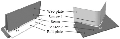
Fig.ô 3
Radius model in top and side view

Fig.ô 4
Measured and simulated temperatures of the straight test specimen, with vS = 40 mm/s
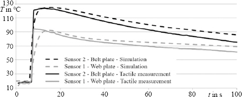
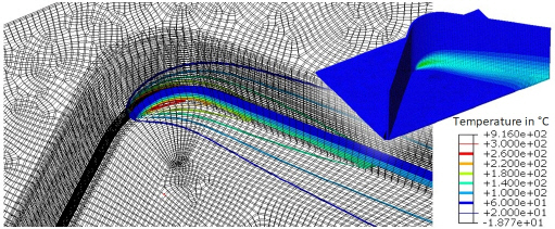
Fig. 5 shows a snapshot of temperature field isotherms, simulated in Abaqus. The view is directed to the root of the weld seam and its elevated temperature. Due to non-linear movement, the heat source enters a higher preheated area. This effect and heat flow from the heat source lead to an increased heat accumulation.
Fig.ô 5
Isotherms of the radius simulation model during the movement of the heat source
The following describes the temperature distribution along the weld seam. The measurement of the temperature is done by a virtual sensor running 20 mm behind the heat source. The determined temperatures over the path of the welds are shown in
Fig. 6. Considered convex radii are
r = 20 mm,
r = 35 mm, and
r = 50 mm. The Fig displays that there is an elevated temperature in the area of the radii. The smaller the radius, the higher the temperature increases.
Fig.ô 6
Simulated temperatures in the weld root, with different outer radii, measured with virtual temperature sensor running behind the heat source
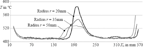
In addition, an elevations at the beginning and end of the path in
Fig. 6 appear from the smaller sheet volume into which the heat flow can dissipate. As the radius increases, the total distance travelled decreases. This is expressed by the earlier start of the temperature rise at the end of the path. The reason for this increase in temperature is the reduced volume into which the heat can flow. Thus, a heat accumulation can also be observed here in the simulation model.
4. Power reduction method
In the last section it was shown that an increase of the temperature in radius r occurs during welding with constant power, which may lead to defects in the weld seam. In the following the increase of the temperature will be explained on the basis of the volumetric heat flux density qV.
The volumetric heat flux density qV is shown in eq. (1) as a function of the heat input and output Q, the related volume V, and the time increment öt. With or without radius, due to constant welding speed, the time increment öt is constant. Also there is no change in heat input Q, due to constant Power PGesamt.
The input power overlaps in the weld root of the radius. Corresponding to the reduced volume into the heat can flow into, the volumetric heat flux density
qV increases. According to the energy balance flow eq. (2) from Anders
3) the increase of the volumetric heat flux density
qV means an increase in temperature
T. This applies for a volume element with side length
dx,
dy, and
dz, the specific heat capacity
c, and density
ü.
In order to reduce the increase in temperature and thus failures in the radius, the heat input has to be reduced. The necessary amount of the reduction is the heat QAdjust, which is based on the power PAdjust. According to eq. (3) the amount of adjustment of the power PAdjust depends on the specific heat capacity c, the mass m, and the temperature rise öTElevate in the area of the radius.
The specific heat capacity c depends on the temperature, increasing degressively with temperature rise. For the range in consideration, the change of the factor is a relatively small compared to the temperature multiplier. The bending of the sheets lead to a constant mass m. Due to the relatively constant heat capacity c, the necessary power adjustment PAdjust is, as shown in eq. (4), approximately proportional to the raise in temperature öTElevate.
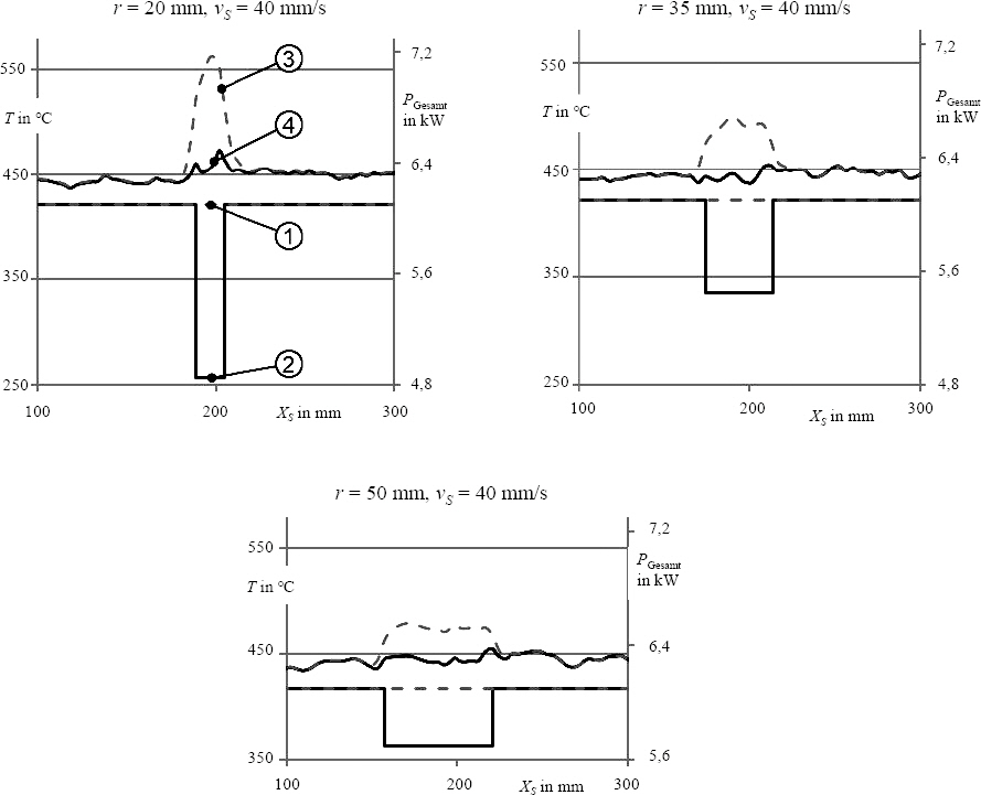
Simulated temperature curves of the radius simulation model are shown in
Fig. 7 for the convex radii
r = 20 mm,
r = 35 mm, and
r = 50 mm. These were simulated with constant and with adjusted power in the radius. Total input power corresponds to the functions ã and ãÀ. The temperatures resulting from these powers are shown in the functions ã and ãÈ.
Fig.ô 7
Total input power PGesamt ã and ãÀ and resulting simulated temperature T ã and ãÈ, depending on the radius r
5. Evaluation and Conclusion
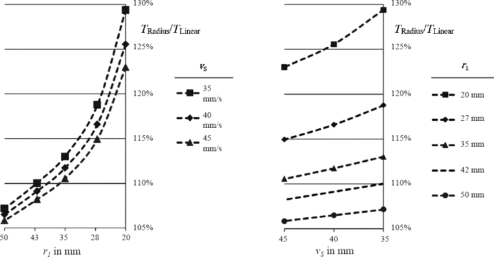
The necessary adjustment of the power becomes higher with smaller radii or lower welding speed. This phenomena can be derived from
Fig. 8. Temperatures of the radius
TRadius are shown relatively to temperatures
TLinear, which are present in linear sections. There are clear excesses of almost 30 %.
Fig.ô 8
Simulated radius temperatures, relative to linear sections. For various radii and welding speeds
In addition, the smaller the radius, the more unsuitable the power adjustment becomes. This can be observed particularly in function ãÈ. A possible explanation for this are temperature overshoots at the end of the radius. This effect results from the abrupt adjustments in power. If the heat source is at the end of the radius, the power is increased again, although the effect of the excessive heat flux density qV is still effective. This means necessary expansion of the adjustment beyond the start and end point of the radius. Due to the heat flow in front and the resulting heat accumulation, the smaller the radius, the larger the expansion must be.
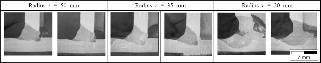
The power reduction method developed through simulation was tested with welding trials on a real part. Cross sections of this trials are presented in
Fig. 9, and show for radii of
r = 50 mm a well working prediction. The intended root connection is reached. For radii with
r = 35 mm one of the two welded specimen show a partial missing root connection. And for the smallest radii of
r = 20 mm, there is a deviation from the desired welding result.
Fig.ô 9
Cross sections of the radius welds with compensated power
Reasons for the deviation could be the remaining overshoot or a drop in welding speed vS in the radii. The smaller the radius, the faster the robot must move with its welding head. A limitation of the welding speed could counteract this. The smaller the radius, the smaller the maximum permitted speed would have to be. Another alternative would be to reduce the height of the laser-MIG hybrid welding head.
In the present work the following points have been shown.
Illustration of 2-D welds of convex radii in the simulation and via real trials.
Function of a virtual sensor, which follows the heat source in the simulation, for the determination of the temperature rise in convex 2-D radius, compared to linear 1-D welds.
Establishment of a power adjustment for the radii, based on a physical model and its real verification.
Display of necessity for further research for a complete automation of the parameter choice for 2-D welds. A radius-specific ramping in and out of the power adjustment would be conceivable.


 PDF Links
 PubReader
 ePub Link
 Full text via DOI
 Download Citation
 Print
Print


