Non-Destructive Testing of Laser Welded Hydrogen Storage Tank Liner Using Optical Coherence Tomography
Article information

Abstract
The Type 4 hydrogen storage tank has an internal liner made of polymer material. Instead of the joining of two cylinder-shaped liners through butt-joint thermal fusion bonding, a faster joining can be achieved through lap-joint laser welding. Non-destructive testing is required to inspect the quality of laser-welded areas and to detect pore defects. In this study, the interface of a laser-welded region is investigated using optical coherence tomography to detect internal pore defects, where the maximum thickness of the liner is found to be approximately 3 mm. Optical coherence tomography images with defects are then used for supervised YOLOv2 deep learning. Real-time detection of internal defects is successfully performed on laser-welded liner samples.
1. Introduction
In the automobile industry, design to increase the efficiency of key components and the development of high-quality manufacturing processes are required to respond to environmental regulations and growing demand for eco-friendly vehicles. To manufacture ultra-high-pressure hydrogen storage tanks, which are key components in hydrogen vehicles, precise welding of internal plastic liners is required. The existing thermal fusion method has similar processes to conventional friction welding. After heating and melting both ends of the liners made of thermoplastic materials using heating plates, the melted surfaces facing each other are pressurized on both sides to perform butt welding. Deburring is then required to remove the solidified liner residue on the outside. Recently, studies have been conducted on laser welding of polymers1,2). Laser welding uses the laser transmission and absorption properties of liners. A white liner is placed on one side and a black liner on the other side so that they can face each other. The black liner is inserted into the white liner to form overlap joints. When a laser beam is irradiated on the surface of the white liner, the beam penetrates through the white liner and is absorbed by the black liner. As the liner is melted by the laser energy and then solidified, the black and white liners are bonded. Since laser welding is faster than the thermal fusion method, it increases productivity. In addition, it does not require deburring. Non-destructive testing of the joint, however, is required because pore defects may occur at the interface while the liner material vaporizes under high heat input conditions.
Optical Coherence Tomography (OCT) is a technology for inspecting the inside of a light-transmitting material by combining the Mikelson interferometer and confocal microscopy. It can obtain the cross-sectional images of a material like an ultrasonic B-scan. Since the inside of materials that transmit the wavelength of the light used in the OCT device can be inspected, OCT has been widely used for the inspection of defects in polymers3,4) and LCDs5), polymer coating material inspection6), and film thickness measurement and defect inspection7). Conventional ultrasonic testing requires contact and contact media, but OCT can inspect the inside while maintaining a certain distance without contacting the material. This study aims to propose a method for detecting defects using OCT and automatically determining defects using deep learning for quality inspection of overlap joints in the liner manufacturing process. OCT was performed in the welding direction and continuously acquired B-scan images were stored in an array. The images were displayed in three dimensions (3D) for the overview of the joint. In addition, the OCT B-scan image samples of joints with pore defects were used for the training of the YOLOv2 object detector. The trained object detector was used to find the positions of defects and display them in real-time while performing OCT for liner joints with pore defects.
2. Testing of Joints Using OCT
2.1 Laser welding process and joint geometry
The liner laser welding process and the joint geometry are shown in Fig. 1. The white liner (liner(white)) is placed on top of the black liner (liner(black)), and they were mechanically pressed to each other to form an interface. When a laser beam that penetrates through the white liner is irradiated, the temperature at the interface increases, thereby melting the liner material. As bonding is performed along the welding direction, the material slowly solidifies and forms the welded area. The unmelted parts on the left and right sides of the joint are left as non-welded areas as shown in the area marked with red dotted lines in Fig. 1(a). No defect occurs under proper welding conditions, but pore defects are formed under high heat input conditions if the liner material vaporizes and it fails to escape from the inside of the welded area. Under low heat input conditions, strength decreases due to the formation of the narrow welded width. Both the white and black liners used in this study had a thickness of 1.5 mm, and the total thickness of the welded specimen was 3 mm.

Cross section view (a) and isometric view (b) of welding process of liner specimen
2.2 OCT device setting and experimental method
An experimental setup was prepared to inspect the cross-section of liner joints as shown in Fig. 2. A specimen was placed on the X-Y stage controlled using a laptop, and an optic head for OCT was located at a certain distance. The optic head was connected to the OCT device. The laser beam for measurement generated from the OCT device is transmitted to the optic head through the optical fiber and then irradiated to the specimen for testing. The B-scan images processed in the OCT device could be viewed in real-time through the monitor. The OCT device used was Lumedica’s OQ Stratascope 1.0. The laser for OCT had a wavelength of 1,310 nm, a maximum power of 2 mW, a scan width of 7 mm, and an A-scan speed of 18,000 /sec. Its magnification could be adjusted by changing the objective lens. The lens used in the experiment had a magnification of 4x. In this case, ROI is 4.6×4.6 mm2. The laser wavelength had to be selected between 1,310 and 840 nm. The transmittance of the white liner to be tested is approximately 0.4 for 840 nm and 0.6 for 1,310 nm, showing that the transmittance for 1,319 nm is 50% higher compared to 840 nm. In other words, thicker materials can be measured using a wavelength of 1,310 nm. The laser power for OCT needs to be properly adjusted by examining the results of B-scan images. If it is too high or too low, cross-section analysis is impossible. It was set to approximately 0.6 mW in this study. The resolution of B-scan images was 512×512, and it had 8-bit gray pixel values. The X-Y stage was orthogonally constructed using Thorlab’s HS NRT100/M (X-axis) and DRV250 (Y-axis). The X-axis direction of the stage was parallel to the welding direction, and inspection in the welding direction was performed by moving the stage along the X-axis.
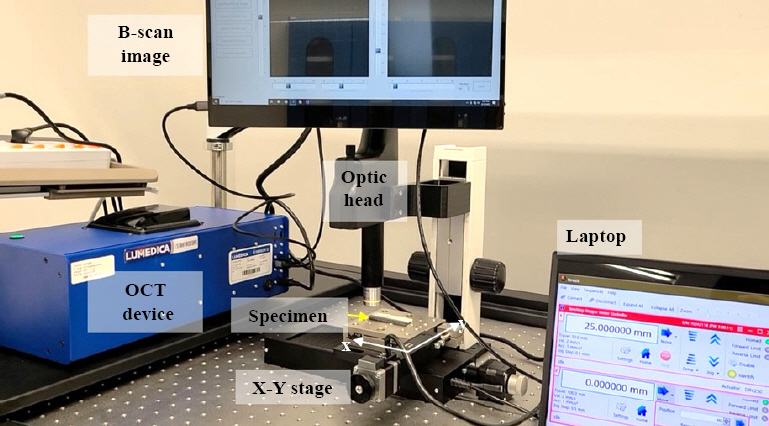
Experimental setup
3. OCT Results
3.1 Identification of the maximum thickness that can be measured
Since the welded area of the laser-welded liner specimen is located 1.5 mm from the surface, it is necessary to identify the thickness that can be measured using the OCT device. For this, white liner specimens processed with a thickness of 1.5 mm and 3 mm were measured using OCT, and the B-scan images were shown in Fig. 3. High image intensity values were observed from the top and bottom surfaces of the specimens. This is because the laser for OCT is well reflected at the boundary of the medium. The top and bottom boundaries of the specimens were clearly observed in the left image with a thickness of 3 mm and the right image with a thickness of 1.5 mm, indicating that the cross-section of laser-welded liner specimens with a thickness of 1.5 mm can also be inspected using the OCT device.

B-scan image of white liner specimen
3.2 OCT measurement for laser-welded joints
Fig. 4 shows the optical microscope, metallurgical microscope, and OCT B-scan images of a laser-welded liner specimen. A defect could be identified in the optical microscope image, but it was difficult to measure the welded width. In the metallurgical microscope image, the welded width, non-welded areas, and pore defect could be observed relatively well. The welded width, non-welded areas, and pore position could also be identified in the OCT image. In the OCT image, non-welded areas can be distinguished, unlike the welded area due to the presence of the gap without fusion. A comparison between the microscope and OCT images shows that non-destructive testing of liner joints is possible using OCT. Unlike Fig. 3, however, the bottom liner of the welded liner specimen cannot be identified because it is black and the laser wavelength used in OCT is absorbed without transmission.
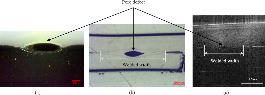
Cross section images of laser welded liner specimen, (a) optical microscope, (b) metallurgical microscope, and (c) OCT B-scan
3.3 3D visualization of the joint using B-scan images
If OCT images are stacked and arranged in the welding direction, the entire internal testing results can be identified in 3D8). To this end, a specimen was placed on the stage and 60 OCT images were captured per second while the specimen was moved at a rate of 2 mm/sec. For 3D visualization, the obtained video was read again by frame and converted into an array using Matlab R2021 from Mathworks. The image array can be returned in 3D using the volshow function provided in Matlab. The rendering style was set to maximum intensity projection. This is the method that has been widely used in medical fields, such as converting brain MRI images into 3D9). As an additional option, Parula was used as the color map of 3D images. Fig. 5 shows the OCT image represented in 3D volume using this method and the specimen used. It can be seen that the pore defect identified in the OCT B-scan image is actually a wormhole defect. The non-welded areas on the left and right sides of the welded area can also be identified at once, and it can also be seen that the welded width varies along the welding direction. Fig. 6 shows the 3D OCT results for the laser-welded cylindrical liner product. An OCT video was recorded while the 316mm-diameter liner was rotated by 360 degrees. 7,200 images were obtained from the video, and volume rendering was performed using maximum intensity projection. Due to the narrow ROI caused by using the lens with a 4x magnification, only the non- welded interface on one side was identified. No significant defect was found inside the joint, and very small pores were scattered between the interface and the welded area.
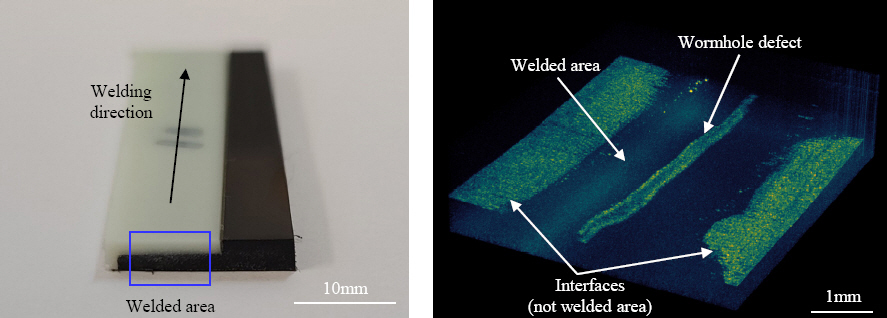
Laser-welded liner specimen and its 3D OCT image
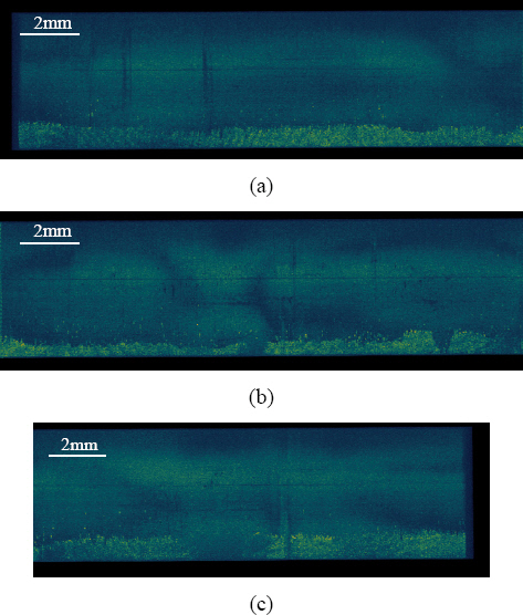
One-third segmented 3D OCT image of a fully inspected circumferential laser welded liner: (a) from start to middle, (b) middle area, and (c) middle to end
4. Real-Time Defect Detection Using Deep Learning
4.1 Preprocessing for deep learning
To detect defects in real-time during the laser welding of the cylindrical liner, the object detection method based on YOLOv2 deep learning was applied. YOLOv2 was announced in 2017, and its performance has been rapidly improved such as by announcing YOLOv8 in 2023. In this study, YOLOv2 was selected because it facilitates the development of an object detector with many reference data. Object detection techniques include Faster R-CNN and SSD512, and YOLOv2 has the benefits of fast processing and high accuracy. In a study by Joseph Redmon et al., YOLOv2 352×352 exhibited 80 frames per second (FPS) and a mean average precision (mAP) of 73.7, but Faster R-CNN (5 FPS and mAP 76.4)and SSD500 (19 FPS and 76.8 mAP) showed slow processing10). Laser-welded liner specimens under various laser welding conditions were subjected to OCT testing, and 105 OCT images with pore defects were collected as shown in Fig. 7(a). Since supervised learning is required for object detection, box labeling was performed for pore defects, which are the targets to be recognized, as shown in Fig. 7(b). YOLOv2 has two subordinate neural networks, a feature extraction neural network and a detection neural network. The feature extraction neural network usually uses pre-trained CNN, and ResNet-50 was used in this study. To shorten the learning time, the size of the images to be used for learning was converted into a resolution of 224×224, which is the minimum size for learning. Among the 105 processed images, 60% were used for training, 10% for validation, and 30% for testing the trained detector. In addition, the number of training images was quadrupled by reversing the left and right sides of the images and changing their brightness and contrast to increase training data as shown in Fig. 7(c).
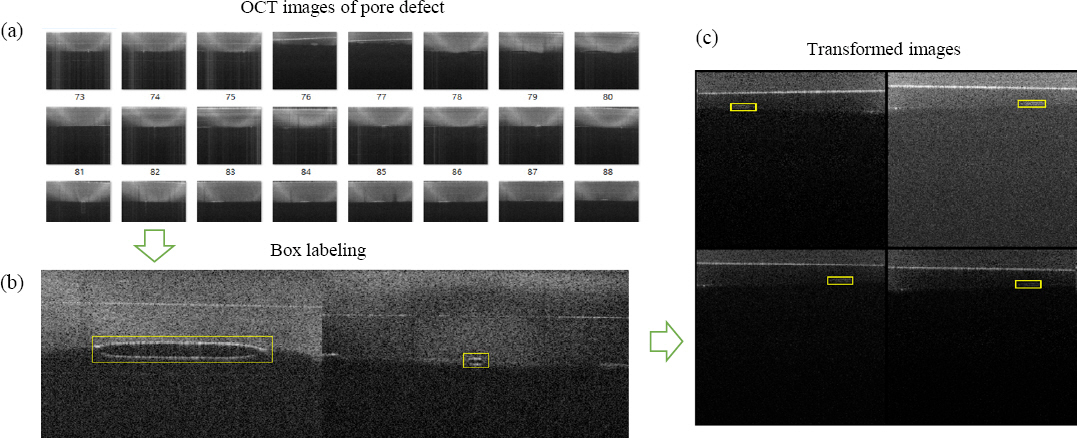
OCT image preprocessing for deep learning
4.2 Neural network learning
Several set values are required for neural network learning. They mainly include the gradient descent type, epoch, and learning rate. The results of training according to them were compared. The common variables used for training are shown in Table 1. The following three gradient descent methods were used for training: Stochastic Gradient Descent with Momentum (SGDM), Root Mean Square Propagation (RMSProp), and Adaptive Moment Estimation (Adam). The results of training performed using each method are shown in Table 2. When the Adam method was used, the average precision was high. Table 3 shows the results obtained by using the Adam method and varying the epoch and learning rate. When the epoch value was doubled from 200 to 400, the average precision and RMSE decreased, but the learning time almost doubled. When the epoch value was fixed at 200 and the learning rate was reduced by half, the average precision decreased and RMSE increased while the learning time did not increase significantly. To examine the occurrence of overfitting according to the epoch value, the training and validation losses were expressed in graphs as shown in Fig. 8. The cases were found to be suitable because the difference in training and validation losses was small, and fluctuating tendencies were similar. Based on these results, Adam was used as the gradient descent method for YOLOv2 training in this study, and an epoch value of 200 and a learning rate of 0.001 were applied. The training data were mixed before each training epoch and the validation data were mixed before each neural network validation to prevent overfitting. The software used for learning was Matlab R2021b, and the PC used for learning had Intel i7-11700K as CPU, Nvidia RTX3060ti as GPU, and 16GB RAM.
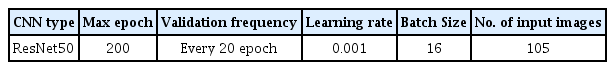
Common variables used in neural network training

Average accuracy and RMSE by gradient descent method type
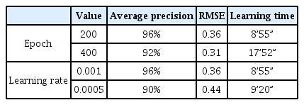
Average accuracy and RMSE by epoch and learning rate with Adam optimizer
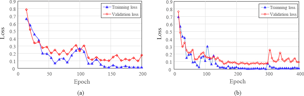
Training and validation loss graph in the case of, (a) epoch value was 200 and (b) epoch value was 400
4.3 Object detection using YOLOv2
Defect detection was performed using the trained neural network for defective specimens that were not used in training, and the results are shown in Fig. 9. As shown in Fig. 2, a laser-welded liner specimen was placed on the X-Y stage and moved in a direction parallel to the welding direction. The OCT image measured at the same time was processed in real-time through the YOLOv2 detector, and the position of the pore defect was labeled using a yellow box along with the probability (%) as shown in Fig. 9(a). For other laser-welded samples, pore defects and their positions were recognized by conducting the defect detection test as shown in Fig. 9(b). 60 B-scan images were acquired per second, and approximately 0.066 seconds were required to determine the position of a defect through the detector.
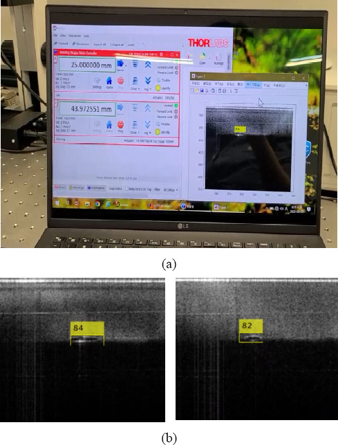
Using a trained neural network for defect detection, (a) real-time continuous defect detection and (b) defect detection results of other specimens
5. Conclusions
In this study, a non-destructive test method was proposed using optical coherence tomography (OCT) for the laser-welded overlap joints of liners, which are structures inside hydrogen storage tanks. The conclusions can be summarized as follows.
1) OCT was performed for liners, and it was found that materials that transmit the wavelength of the light emitted from the OCT device can be inspected to a depth of up to 3 mm.
2) OCT and microscope cross-section analysis was conducted on pore defects that occurred in the welded area. The welded width, pore defects, and non-welded areas were examined using the B-scan images obtained through OCT, and they could be identified at a level similar to that of microscope images.
3) The internal geometry of the entire joint was displayed by performing three-dimensional (3D) rendering of OCT images using maximum intensity projection so that the welded area and defects could be inspected at once.
4) Supervised learning was performed with OCT images containing pore defects for automatic defect detection using YOLOv2. For random specimens with defects, the trained neural network detected defect positions in real-time.
Acknowledgement
This work was supported by the Global Core Industry Quality Response Root Technology Development Program of the Ministry of Trade, Industry and Energy (No. 20016020) and the Basic Program of the National Research Council of Science and Technology (No. NK244A).